About a year ago I finished up a year of doing machine learning research at Google as a Google AI Resident. Technically when I started I was a Google Brain Resident, but midway through the powers that be decided to rebrand the program and thereafter I was supposed to refer to myself as a Google AI Resident. I was in the second cohort so the program as a whole was still having a few teething issues, but it was nevertheless an extraordinarily valuable experience. This is a (fairly lengthy) blog post about my time there.

Application and interview

I think I first heard about the Google Brain Residency from one of Jeff Dean’s tweets and decided to apply almost on a whim. The cover letter was probably the most important part of the application. I treated it almost like a short research proposal, starting with some unifying threads in my past work and explaining how they were motivating the questions I wanted to answer at Google and why Google would be a great place to try to solve those problems. In my case I had been working at a company called Persyst that does machine learning to interpret EEG data. Most of my work there had been working with EKG data to robustly identify heart beats in noisy conditions. Heart beats can be picked up by the EEG and look very similar to a feature that is characteristic of epilepsy and could confuse the other classifiers.

I was trying to build a system that would be robust to novel conditions and I started thinking more generally about the problem of how to determine if a data point is similar to things a neural network (NN) has seen before, or if it’s wildly different. This is distinct from (though related to) the problem of calibrating the uncertainty of a NN. As an illustration, imagine a NN that was trained to classify handwritten 1s and 0s. If you give the NN a very narrow 0, it will return a confidence of around 0.5. But if you provide the NN with white noise then it will still probably return a confidence of 0.5 even though this example is quite different than a narrow 0. Unfortunately just rejecting anything that’s classified with a confidence close to 0.5 isn’t good enough because you can easily come up with unusual data that the NN will classify into one or the other classes with high confidence. If you give the NN the letter “t”, for example, it will probably think that looks much more like a 1 than a 0 and so will classify it accordingly with high probability. Adversarial examples are the extreme limit of this out-of-distribution problem where you manage to construct an example which perceptually belongs to one class, but the NN classifies in another with high confidence. I wasn’t exactly sure how to go about solving this problem (it’s hard!), but it was one of the things I was thinking of at the time. In the end my research at Google Brain turned out to be on completely different topics though I’m still interested in this problem.

I was fortunate to be selected for a phone screen where I was interviewed by Kevin Murphy. The phone screen mostly focused on the machine learning work that I had done and delved a little bit into what I wanted to do at Google. The phone screen went well and I was selected for an onsite interview in late February. During the onsite we were given a tour of Google Brain (they had some robots running around, which made it especially cool!), and got to see a few short presentations by Brain Residents from the previous cohort about their research. But of course the reason we were all there was for the interviews. The interview had two components: a machine learning interview and a programming interview. I thought that the programming interview went okay, though not great, but I thought that I had completely bombed the machine learning interview. When I got home I was happy that I had gotten as far along in the interview process as I did, but was fully prepared to receive a rejection. But to my surprise about a month later I heard that I had been accepted!

Orientation

There ended up being about 30 AI residents in my cohort. As AI Residents we were technically “fixed-term full time employees” (so, not contractors or interns). As such in mid-July we went through the Google’s normal two-day employee orientation. After this we had a separate orientation specific for AI residents that lasted about three weeks. Each of us got an “orientation mentor” who showed us the ropes about how to do basic things within Google Brain. (There were varying degrees of helpfulness from the orientation mentors. My mentor, Patrick Nguyen, was great, but I think some residents never saw their orientation mentor at all.) Chris Olah also taught a crash course in deep learning for us.

During this time we chose a topic for a “mini-project” that we would do to get familiar with Tensorflow and Google’s infrastructure. In my case I decided to train a model to generate captions for New Yorker cartoons. It turned out that someone at Google Brain (Chris Shallue) had already done a project like this, so some code was already available. My plan was to add some more data to the training set to see if the results improved.

Sadly, the model I trained didn’t really learn to make clever New Yorker cartoon captions, though perhaps that was asking a bit much of it given that there are only 80,000 or so New Yorker cartoons in existence. It really just ended up learning that a fine start to nearly any New Yorker cartoon is “I’m sorry sir, but…” Any amusing captions it produced was purely by coincidence. But there wasn’t really enough time in two weeks to do much experimentation, especially with the other orientation activities going on.

Towards the end of our orientation we attended a series of presentations to help us decide which research projects to embark on during the residency. Research scientists would give us a five minute pitch about different projects they wanted a resident to work on. After a few days of presentations (and over a hundred research ideas!) we had some time to go over the different projects and talk to the people we’d potentially work with before deciding on a first project.

Research

After about three or four weeks our schedule freed up considerably so that we could spend most of our time on research. We had been encouraged to choose only one research project, but it was really challenging to limit oneself to just one and I ended up choosing two. I’ve personally found that having two projects going simultaneously is helpful because you can usually make progress on one when the other has stalled for a little bit (or you’re just sick of it).

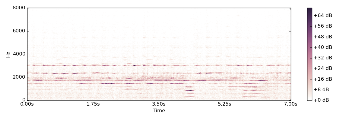
Audio textures

The first project I chose was to generate audio textures with Matt Hoffman and Ron Weiss. The idea was to take a short clip, say 10 seconds, of some “textured” audio like a crowded cafe or a babbling brook, and then generate a new audio clip which sounds similar to the original. The project seemed fairly straightforward since Gatys et al. (2015) had shown that the features of a deep neural network could be used to generate image textures that were far more sophisticated than anything that had been done previously. There had been some earlier work done in audio texture synthesis by McDermott & Simoncelli (2011), but it had predated the recent advances in deep learning and used a complicated set of hand-crafted features. It seemed natural enough that we would be able to extend the neural texture synthesis technique to audio and would similarly get much more sophisticated textures.

As I embarked on this project I started doing some more background reading and quickly discovered that Dmitry Ulyanov and Vadim Lebedev had written up a really cool blog post that extended the neural texture synthesis technique to audio. I was able to reproduce the results from Gatys et al. (2015) on image textures and Ulyanov & Lebedev’s work on audio textures within a week or two, but I wasn’t particularly happy with the results on certain kinds of textures. In particular bells with long, sustained tones did not sound very good, nor did any textures with rhythmic content.

Given the current state of the art, I figured there was enough room for improvement to make pursuing this project worthwhile, so I started to experiment with some different ways of getting the harder textures to sound good. I had some early successes here by combining a few known techniques in the literature for image texture synthesis, such as using a set of convolutional filters with varying widths (a technique developed by Ustyuzhaninov et al., 2016). This produced much higher quality audio for bells. Furthermore, one of my mentors pointed me to a paper by Sendik & Cohen-Or (2017), which had used the autocorrelation function as a feature that allowed them to produce textures with regular patterns like a brick wall. I found that I was able to use this feature to produce audio textures with rhythm like a person tapping. By the end of October I was pretty happy with the quality of the textures that were getting generated.

A diversion into spectrogram inversion

As I was going down this path I started to think more deeply about the question of how to invert a spectrogram. It is fairly common in the audio world to work with spectrograms rather than raw audio because it’s much closer to how our brains actually interpret an audio signal. If you’re trying to generate audio, the power of this representation makes it natural to generate spectrograms as an intermediate step, but you’ll ultimately need to somehow go from that spectrogram to raw audio so you can listen to the results. The problem here is that the spectrogram only considers the magnitude of the STFT of your signal — all the phase information is thrown away. In principle this isn’t actually a problem because as long as the hop size of your STFT is less than or equal to 50% of your window size, there’s enough redundant information in the spectrogram to perfectly reconstruct the original audio signal (modulo some global phase difference). But in practice, finding that audio signal is too difficult. Moreover, if you’re using some ML algorithm to generate a spectrogram, there’s no guarantee that any audio signal actually corresponds to your spectrogram.

For the past 35 years, the standard technique for inverting a spectrogram has been the Griffin-Lim algorithm. The idea is to start with random phases in each of the STFT bins, and then go back and forth between spectrogram and audio, updating the phases so that the spectrogram of the resulting audio more closely corresponds to the original spectrogram. The result will generally sound okay, but will contain audible artifacts. Moreover Griffin-Lim is pretty slow, usually requiring a few hundred iterations for a solution to converge. For my ten second audio clips that would take a few minutes to go from spectrogram to audio. There have been a few variants on the Griffin-Lim algorithm over the years (mostly aimed at making it faster), but there haven’t really been any qualitative improvements in the resulting audio.

I thought that deep learning could provide a way to invert spectrograms with much higher quality. And I certainly wasn’t the only person thinking along these lines! At the time Jonathan Shen was working on Tacotron 2 and got really good results for text-to-speech for the Google Assistant voice by conditioning Wavenet on a mel spectrogram. I was curious, though, if this technique could be made more general. What if, instead of synthesizing a single speaker’s voice, we could produce any audio by conditioning Wavenet on its spectrogram?

I ended up spending about two months following this line of thought, unfortunately without much success. My idea was to use AudioSet as a dataset of “general sounds” and to try to train Wavenet to reproduce those sounds by conditioning it on the spectrogram of those sounds. In the spirit of my original project of audio texture synthesis, I also tried to train Wavenet to generate sounds from AudioSet unconditionally with the idea here being that you could give this Wavenet some audio texture and have it extend the texture indefinitely. Sadly the resulting audio was very low quality (there was always a pretty loud buzz that I wasn’t able to get rid of), and synthesizing audio from Wavenet was painfully slow, which made rapid iteration impossible. My mentors and I even mused a little bit about going further afield from the original project by looking into whether we could speed up Wavenet synthesis, but dropped the idea after we heard that a team at Deepmind was about to release Parallel WaveNet, which did just that.

While I ended up learning quite a bit about deep learning for audio from this diversion, those two months ended up wasted from a performance review standpoint since I couldn’t point to any artifacts (Googler-lingo for a paper, presentation, codebase, or some other kind of document) that resulted from that work. In retrospect, trying to get Wavenet to learn all of AudioSet unconditionally was probably asking a bit much of it given the diversity of audio (and audio quality!) in that dataset. I’m still of the opinion, though, that with more work I could have gotten some variant of Wavenet working that would invert general spectrograms. But a year is not a long time and I had to prioritize the work I wanted to do for the rest of the residency. Taking a risk for a few months was fine, but given that this gamble had failed I had to retreat and work on something safer in the remaining time.

Writing the paper

By this point it was mid-December and the submission deadline for ICML was coming up in early February. We wanted to have some tangible results from this project, so we decided to prepare a submission. From a career perspective, this was also something of a necessity for me since the timing of the conference deadlines meant that ICML was the only major conference for which I would get a decision before the end of the residency.

The main shortcoming in the audio textures that I was able to generate at this point was that there wasn’t a lot of diversity in the results. I tried addressing this by adding a diversity term to the loss from Sendik & Cohen-Or (2017) that would penalize the algorithm for producing a texture that was too similar to the original, but the algorithm would sneak around this by reproducing the original exactly, but shifted over in time by a few seconds. I ended up solving this issue by changing the loss term so that the algorithm was penalized for reproducing something too close to the original shifted by any amount of time.

We felt that the quality of the audio textures was good enough by now to start writing up an ICML submission. The hope was that by combining a scattered set of techniques for texture synthesis in the literature (e.g., multiple receptive field sizes, random filters, an autocorrelation term), plus developing an improved diversity term, along with substantial quantitative and qualitative analysis of the results, we would have a paper that would be sufficiently interesting for ICML. The reviewers ended up giving us generally positive reviews about the paper and the quality of the audio textures, but as expected the main criticism was that the work just felt too incremental for ICML. And honestly I think they were right. The paper was rejected, so we incorporated some of the reviewers’ suggestions and later submitted it to TASLP, where it was again rejected for similar reasons. After that we submitted the paper to ICASSP 2019, where it was finally accepted, though at about half the original length and without most of the analysis. (The original, full-length paper can be found here.)

Batch size

Concurrent to my work on the audio textures project I also started on a project to study the effect of batch size on training time. There had been some papers in the literature arguing that neural networks trained with larger batch sizes generalize worse, but other researchers had argued that you could achieve the same performance by increasing the batch size so long as you also increased the learning rate. The goal of this project was to do a thorough set of experiments on a wide variety of tasks and architectures to determine what the relationship really was between batch size, training time, and generalization, controlling for hyperparameters as much as possible. George Dahl conceived of and managed the project, and he recruited Jaehoon Lee and myself to actually carry out the experiments.

I liked this project from the start because I was (and still am) of the opinion that the machine learning field has too few systematic studies, and as a consequence there is a lot of cargo culting. I also thought that it wouldn’t take a huge amount of time — how hard could training a few models and varying the batch size be? But as we began it became clear that this was much more technically complicated than we originally anticipated.

Our original idea was to use the tensor2tensor library for the project since they had implemented a variety of models that could train on a variety of different tasks like image classification and neural translation. Unfortunately, for this project we needed absolute control over exactly how many examples went into each training step and on the language models this turned out to be very difficult in tensor2tensor. Around this time George had recruited Chris Shallue to help us out as a technical lead. We tried working with tensor2tensor for a bit, but soon decided it would be more efficient to write our experiments from scratch. Chris built an experimental framework that used Vizier to manage the experiments we ran, Jaehoon worked on the language model experiments, and I was tasked with running the image classification experiments.

During this project I encountered the most difficult bug I’ve had to deal with in my career. I had implemented ResNet-50 for the ImageNet task, and it was known that with a certain set of hyperparameters, the model should obtain an accuracy of just over 75%. Yet I consistently saw that I was getting just over 74%, about 1% less than I should. I spent about a week debugging this on and off on my own, but made little progress because the model took about 8 hours to train even on a TPU.

Ultimately I ended up spending a few days with Jaehoon and Chris where we went layer by layer and compared the network output with a reference implementation. Mysteriously, every layer matched and the overall output was the same as well. Moreover, every contribution to the loss we could find was identical as well, although the overall loss was slightly different. After more digging Chris discovered that weight decay was getting applied to every layer except for the very last softmax layer because the softmax layer was applied in a separate module. The weight decay on that single layer turned out to be key and was the difference between 74% accuracy and 75% accuracy.

Once that bug was fixed the rest of my contribution to the project was mostly running and organizing a large number of image classification experiments. For every batch size I would train \(\sim\)100 models with a variety of different learning rates and momenta. Building the infrastructure for this project took until about February, and the experiments took another four months or so to run. (This was a computationally heavy project even by Google’s standards.) By the time I left the residency we had just about collected all our results and had decided to submit to JMLR since there were enough results that it would be too awkward to try to fit them all in a conference paper. Unfortunately since I was outside of Google when the writing began I didn’t get to be one of the first authors on the paper, which was a bit of a bummer. But I am very happy with the quality of the results. It was one of those projects that could really have only been done at Google and I’m glad I got to be a part of it. I am also very grateful I got to work with Chris on the project since I learned an enormous amount about how to design an architecture for a complicated machine learning problem.

PCA of random walks

After I had submitted my audio textures paper to ICML I had more free time on my hands. I had been following along with some of the work trying to apply techniques from statistical physics to understand neural network training, but hadn’t had the opportunity to do any research along those lines myself. I’m not exactly sure how I got onto this subject, but as I was looking through some of this research I started playing around with random walks as a model for neural network training. While it might sound a little crazy to take the training process which is very much not a random walk and approximate it with something so simple, there is a substantial stochastic component to neural network training.

As I was playing around with high dimensional random walks I somehow noticed that when you apply PCA, you end up getting very smooth curves. Not only are these figures smooth, they are completely regular. I generated a dozen random walks and obtained identical curves after doing PCA every time (modulo an overall sign flip). I thought this was very strange and started to spend a lot of time trying to understand exactly what was going on, perhaps a bit obsessively.

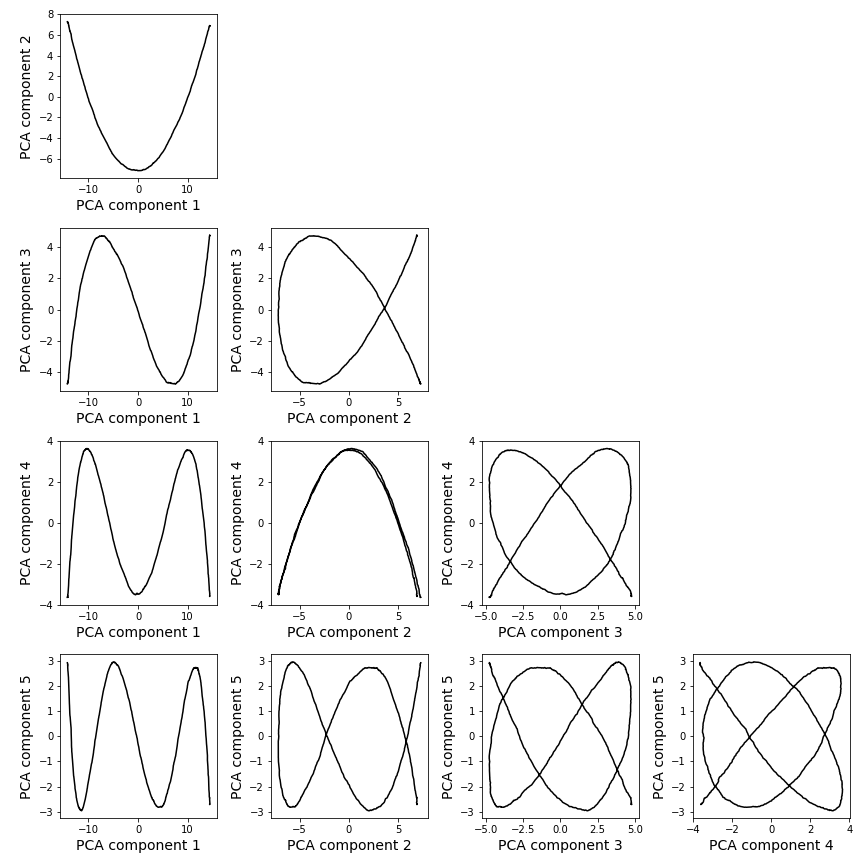
When I had first seen these curves they immediately looked like Lissajous curves to me, so I spent a little while trying to fit them to see if I could find the functional form of the curves. After a little bit I realized that everything was quite simple if I replaced the sines in the Lissajous curve definition with cosines.

I also started to do a bunch of background reading about random walks and quickly discovered an amazing paper by Moore et al. (2018). They analyzed a random walk in the limit of infinite dimensions and showed that when you applied PCA, about 60% of the explained variance is in the first PCA component, and 80% is in the first two! This blew my mind. I compared the distribution of variances that they predicted with what I saw and found that it matched exactly. But they didn’t look at what the random walk looks like when projected onto PCA components. In fact, as I went through the literature, it seemed that no one had looked at this. One paper had noticed that they got Lissajous curves when they applied PCA to their dataset, but no one had made the connection to random walks.

I went through Moore et al.’s analysis step by step to see if I could extend it to show why the projection of the walk onto the PCA basis would always be a Lissajous curve. I was simultaneously talking about random walks to anyone who would listen. Fortunately one of the people who was willing to listen to me was Jascha Sohl-Dickstein, and he pointed out to me that the matrices I was working with were close to being circulant matrices, and that the eigenvectors of circulant matrices are Fourier modes. This it turned out to be a key insight. With some more effort I was able to work out a derivation that showed that the projection of a high dimensional random walk onto the PCA components would be a Lissajous curve.

During this time I was continuing to do more background reading and had found that a number of authors had tried to visualize neural network training by performing PCA on the model’s parameters over the course of training. In every case they had obtained a smooth, parabolic curve. I had been staring at Lissajous curves for long enough now that I realized that this is exactly what you would get from a random walk. I trained a small neural network on MNIST and projected the weight trajectory onto all pairs of PCA components up to the fifth and found that every combination was exactly the same Lissajous curve one would expect from a random walk.

By now it was late April and I was spending almost every spare moment on random walks. The NeurIPS deadline was in just a few weeks, and I figured I had nothing to lose by trying to collect these results into a submission. I felt that it had a reasonable chance of acceptance since there was a new theoretical result, it explained some results in a recent trend of visualization, and, if I could get it done in time, there would be some good computational experiments to verify the connection with neural networks.

In the last couple of weeks I tried scaling up the neural network experiments to ResNet-50 trained on ImageNet. Conveniently I had already implemented this network for the batch size project so the main difficulty was getting all the parameters out over the course of training. The network trained for 150,000 steps and it had millions of parameters so it was going to a nightmare to try to store absolutely everything (not so much because of the storage space, but writing to disk on every step would slow down training enormously). I decided to break up training into 1500 steps at the beginning, middle and end of training to make things a little more reasonable. Even then, performing PCA on the full set of parameters was prohibitive. I realized, though, that I could take advantage of the Johnson-Lindenstrauss lemma and randomly project the parameters down onto a lower dimensional space, but still preserve the structure. Unfortunately, due a bug in my random projection code I wasn’t able to get results on the entire set of parameters for ResNet-50, so I had to restrict myself to the parameters in a single layer in the initial submission (which also produced a Lissajous curve). But after submitting the paper I was able to fix the bug and got a beautiful set of Lissajous curves for the entire parameter set of ResNet-50 which made it into the final version of the paper.

Ultimately this paper was accepted to NeurIPS 2018. By the time the conference came around the residency was over and I had left Google so I had to pay my own way to present the paper. But it was worth it to talk to yet more people about random walks and catch up with the other residents.

Coming to an end

The question of what to do with us after the residency ended seemed to be the part that Google had thought through least. Officially, the story was that once the residency was over that was that and you’d leave Google. Unofficially, however, the people running the program were expecting most of us to convert to full time positions at Google once the residency ended. This tension between the official and unofficial version made things difficult because it was unclear what the real requirements for conversion were. The stated requirements of the program were pretty minimal — you just had to do machine learning research for a year. There was no expectation of publication or any real results. But it was obvious that if you produced no publications in a year you would not be able to convert.

Some of the residents had a background in machine learning research and so already had a publication record they could point to in support of their conversion process. They also tended to have some projects in the works when they started and were able to get out publications earlier in the program which made it easier for them to convert to research scientist positions at the end of the year. Others like myself were coming from other fields and so we didn’t have an ML publication record yet. Since the residency was only a year long, most of us had a few papers which had been submitted to different venues, but due to the timing of the conference submission processes, it was hard to have more than one accepted paper by the end of the residency. (And because my audio textures paper had been rejected from ICML I didn’t have any).

The recommendation for those of us who didn’t have many publications yet was generally to extend the residency for another year before trying to apply for a research scientist position. Another alternative was to apply for a research software engineer position (called rSWEs in the Googler lingo). Within Google Brain projects are normally conceived of by research scientists and rSWEs will move between different projects to implement the experiments when they require more infrastructure. In practice rSWEs within Google Brain have a lot of freedom to work on research projects that they find interesting. I wasn’t especially keen on extending the residency, mostly for salary reasons. (Residents have a base salary that’s somewhat comparable to a SWE of an equivalent level at Google, but they don’t get any of the stock or profit sharing that makes up a substantial component of a normal Googler’s total compensation.) I had written a fair amount of code for the batch size project, so I decided to apply for an rSWE position.

People at Google will often put up flyers in prominent locations advertising events and open positions. From one of these flyers I learned of an interesting new project to apply ML to meteorological data. The project was going to use a new, untapped data source and I felt I’d be well suited for it given my background in physics. There was a pretty clear use case for an associated product (always helpful for performance reviews at Google), and the project was just getting started, so it would be easy to make significant contributions. I talked to the engineer who was organizing the project and he thought I was a good fit, so I formally applied for the position. As a resident I only had to do two interviews rather than the usual five since I could point to my performance reviews in my conversion packet.

I was simultaneously applying for a number of jobs outside of Google. We quickly learned that it was wise to look outside of Google even if your goal was to remain at Google. Google will be content to string you along and extend the residency as long as possible, so sometimes you have to force their hand with an offer letter from another company. Fortunately, having the magic dust of the Google name on your resume definitely helps you to get noticed by recruiters, but it’s no guarantee of a job! I think I only heard back at all from maybe a quarter of the jobs I applied to. I also reached out to the CEO of a startup called Whisper whom I had met earlier in the residency. Back in September, he had contacted me through a mutual friend and pitched me his idea of using deep learning to do noise reduction in hearing aids. It was a great idea with a lot of potential, but I had only been at Google for two months at the time, so I demurred. But now that the residency was coming to an end, I reached out to him to see how the startup was going and asked if they were still looking for ML engineers. They were, so I interviewed with them and a few days later I got an offer.

This offer put me in a bit of an awkward position with respect to my ongoing application with Google. I knew that it would be at least a month before they made a decision, so I had to decide whether to accept the startup offer or decline and hope that I got an offer from Google and continue to pursue applications at other big companies. Because of the timing of my interviews I wasn’t able to leverage any offers against any others like some of the other residents, although I don’t think that would have been a huge help in my situation since an offer from Google is not really comparable to a startup offer. The startup will say that, well, of course we can’t meet Google’s base salary, but look at how much your stock options will be worth when we’re a billion dollar company! and Google will easily beat the startup’s base salary and will value the stock options at exactly $0. Ultimately I ended up deciding to work for the startup (and I’m still here a year later). I figured that good startup ideas come along rarely enough that it was worth taking a gamble. If things don’t work out the Googles of the world will always be hiring in the future.

One crucial mistake I made after I signed the startup’s offer letter was to tell my manager. I wanted to withdraw my application for the rSWE position at Google so that the project manager for the job I was applying to could move on to other candidates. But she told me that by signing an offer letter for another company I could be terminated and forfeit the bonus you get at the end of the program. A few days later she said she had discussed with some higher ups and said that I could keep the completion bonus (although I learned a few months later that I had to pay back a portion of my signing bonus). I was a bit tired of Google’s antics by now and decided to leave the residency two weeks early and get a head start at Whisper.

As it turned out I was the only resident to leave Google for another company. Most of the residents who didn’t have PhDs went to grad school, and the rest either extended the residency for another year or converted to a research scientist or rSWE position. Although I’m not doing fundamental ML research for my day job anymore, the things I learned during the residency were extremely helpful for my current work at Whisper. I had been self-taught in ML, but there’s only so much you can get by reading books and papers on your own. There’s no substitute for talking with researchers who are at the frontier of our knowledge. And beyond the value the residency had for my own growth as an ML practitioner, the group of researchers and residents that I got to know over the year were among the smartest and kindest people I have met, and it was a true privilege to have worked and become friends with them.