In this article we’ll learn how to train a neural network to play Tic-Tac-Toe using reinforcement learning in Jax. This article will aim to be more pedagogical, so the code we’ll end up with won’t be super optimized, but it will be fast enough to train a model to perfect play in about 15 seconds on a laptop.

Code from this page can be found at this Github repo as well as in a Colab notebook (although the Colab notebook runs considerably more slowly).

Playing Tic-Tac-Toe in Jax

Before we get to the fancy neural networks and reinforcement learning we’ll first look at how a Tic-Tac-Toe game might be represented using Jax. For this we’ll use the PGX library, which implements a number of games in pure Jax. PGX represents a game’s state with a dataclass called State. This dataclass has a couple of fields:

• current_player: This is simply a 0 or a 1 and alternates on every turn. What is perhaps confusing about this is that there is no relationship between player 0 and an X or an O. Player 0 is randomly assigned X or O on each game and X always goes first. This is helpful because it means that you can assign your neural net to always play as Player 0 and ensure that it plays as X (and goes first) half the time and plays as O (going second) half the time.

• observation: This tells us what the board looks like at the current step. The representation PGX uses is a boolean array of shape (3, 3, 2). The first two axes represent the 3x3 grid as you might expect, and then the first channel of the last axis is True wherever there is a piece for the current player and the second channel is True wherever there is a piece for the opponent. (Note that the axes switch on every turn since the current_player switches.) For example, here is a state that the board might be in:

  

  This gets represented as:

Array([[[False, False],
        [False,  True],
        [False,  True]],

       [[False, False],
        [ True, False],
        [False, False]],

       [[ True, False],
        [False, False],
        [False, False]]], dtype=bool)

• legal_action_mask: This is a (flat) boolean array that with a False for every filled space and a True for every empty space.

• rewards: This array is of shape (2,) and gives us the reward on each step. The first index gives us the reward for player 0 and the second for player 1. Note that the reward is provided for the state after a winning move is played. This means that we have to take into account the fact that the current player switches when determining the reward. Rewards are also not cumulative — if we continue to transition to new “states” after the game has ended (which happens due to batching), the rewards on subsequent states are 0.

• terminated: This is simply a boolean value telling us whether the game is over. (PGX also provides an attributed called truncated which indicates that the game ended for some other reason than the game ending normally, e.g., a time limit expired.)

PGX then provides us with a function called step which takes a state and an action and transitions us to the next state. In the case of Tic-Tac-Toe action is very simple — it is just the index of the space we want to lay a piece in. (The numbering goes left to right and then top to bottom, so the top left square has index 0, the top right has index 2, and the bottom right has index 9.)

Finally, because PGX implements all the game logic in Jax, we can run multiple games in parallel, so all of the properties of a state can acquire an additional batch index. This can speed up training considerably.

A random game

To see how this all works, let’s write some code to play a game by making random moves. First we’ll write a function to select a random legal move:

import jax
import jax.numpy as jnp

@jax.jit
def act_randomly(rng, state):
    probs = state.legal_action_mask / state.legal_action_mask.sum()
    # This will be 0 for all legal moves, and -inf for illegal moves.
    logits = jnp.maximum(jnp.log(probs), jnp.finfo(probs.dtype).min)
    return jax.random.categorical(rng, logits, axis=-1)

Now we can run through a batch of games:

import pgx

def play_random_game(rng, batch_size):
    env = pgx.tic_tac_toe.TicTacToe()
    init_fn = jax.vmap(env.init)  # This batches the environment.
    step_fn = jax.vmap(env.step)
    
    key, subkey = jax.random.split(rng)
    keys = jax.random.split(subkey, batch_size)
    
    state = init_fn(keys)
    states = [state]
    
    while not state.terminated.all():
        key, subkey = jax.random.split(key)
        random_actions = act_randomly(subkey, state)
        
        state = step_fn(state, random_actions)
        states.append(state)
    
    return states

If we run this on a batch of 9 games we get play that looks like this:

Clearly not optimal! Let’s see if we can use reinforcement learning to do any better.

A Deep Q Network for Tic-Tac-Toe

The first thing we’ll do is set up the architecture for the neural network. Tic-Tac-Toe is not a very difficult game to learn so this architecture does not need to be very sophisticated. A fully connected network with a couple of hidden layers will do. PGX represents the board state as an array of shape (3, 3, 2), but we can flatten this to an array of length 9. We will put a 1 anywhere there is an X and a -1 anywhere there is an O.

The output of our little neural network will just be a value that the neural net assigns to each space on the board. These values will range from -1 to 1, with 1 implying a high likelihood of winning, and -1 implying a high likelihood of losing. So the output will also be an array of length 9.

Our architecture looks like this:

from flax import nnx

BOARD_SIZE = 9

class DQN(nnx.Module):

    def __init__(self, *, rngs: nnx.Rngs, n_neurons: int = 128):
        self.hparams = hparams
        self.linear1 = nnx.Linear(BOARD_SIZE, n_neurons, rngs=rngs)
        self.linear2 = nnx.Linear(n_neurons, n_neurons, rngs=rngs)
        self.linear3 = nnx.Linear(n_neurons, BOARD_SIZE, rngs=rngs)

    def __call__(self, x): 
        x = x.astype(jnp.float32)
        x = x[..., 0] - x[..., 1]  # Represent X with a 1, O with a -1
        x = jnp.reshape(x, (-1, BOARD_SIZE))
        x = nnx.relu(self.linear1(x))
        x = nnx.relu(self.linear2(x))
        return nnx.tanh(self.linear3(x))

If we want to use a neural network to play a game, all we have to do is select the space that the neural net assigns the highest value. (Note that because our neural net always produces 9 outputs we need to mask out the values associated with any positions on the board that are already occupied.)

@jax.jit
def select_best_action(state, policy_net):
    logits = policy_net(state.observation)
    return jnp.argmax(
        logits * state.legal_action_mask
        + jnp.finfo(logits.dtype).min * ~state.legal_action_mask,
        axis=-1,
    )

Evaluating the model

Even though we haven’t figured out how to train our model yet, we now have everything we need to at least evaluate how well it does against a random player. We can track the model’s performance with a dataclass that stores the number of wins, losses, and ties and displays them nicely for us:

@dataclass
class GameStatistics:
    n_wins: int 
    n_ties: int 
    n_losses: int 

    @property
    def games_played(self):
        return self.n_wins + self.n_ties + self.n_losses

    @property
    def win_frac(self):
        return self.n_wins / self.games_played

    @property
    def loss_frac(self):
        return self.n_losses / self.games_played

    @property
    def tie_frac(self):
        return self.n_ties / self.games_played

    def __repr__(self):
        return (
            f'Wins: {100 * self.win_frac:.2f}%  '
            f'Ties: {100 * self.tie_frac:.2f}%  '
            f'Losses: {100 * self.loss_frac:.2f}%'
        )

Now to measure performance we simply run a batch of games. Whenever current_player is 0 we’ll use the best action as chosen by the neural net, and whenever current_player is 1 we’ll sample a random action. PGX randomly assigns player 0 to Xs and Os, so this will fairly measure the model’s performance going first half the time and second half the time.

Note that because each batch will have a mix of games where the current player is 0 and 1, we’ll want to select the actions for some of the games randomly and select actions using the neural net for the other games. However, in Jax it is generally faster to simply do both for all the games and then mask out the ones we don’t want rather than trying to be clever and only run the neural net for the games where it is necessary. (Even though we are running our neural net twice as often as we need to this is still faster than trying to run a conditional.) In other words, we’ll choose random actions for all the games and also use the neural net to select the best actions for all the games, and then we’ll simply use a mask to combine the two appropriately:

actions = (
    random_actions * state.current_player
    + best_actions * (1 - state.current_player)
)

Running through the loop of a game and tracking the wins and losses, we have a function that looks like this:

def measure_game_stats_against_random_player(
    key, init_fn, step_fn, policy_net, n_games: int = 1024
) -> GameStatistics:
    n_wins = 0 
    n_losses = 0 

    key, subkey = jax.random.split(key)
    keys = jax.random.split(subkey, n_games)
    state = init_fn(keys)

    while not (state.terminated | state.truncated).all():
        key, subkey = jax.random.split(key)
        random_actions = act_randomly(subkey, state)
        best_actions = select_best_action(state, policy_net)

        # Policy net is player 0, random player is player 1.
        actions = ( 
            random_actions * state.current_player
            + best_actions * (1 - state.current_player)
        )

        state = step_fn(state, actions)

        # Since the policy net is player 0, we want the rewards in the 0 index.
        n_wins += jnp.sum(state.rewards[:, 0] == 1)
        n_losses += jnp.sum(state.rewards[:, 0] == -1) 

    n_ties = n_games - n_wins - n_losses
    return GameStatistics(
        n_wins=n_wins,
        n_ties=n_ties,
        n_losses=n_losses,
    )

Ultimately we’ll expect that the model should never lose to a random player (though it sometimes may tie).

Training the neural net

We’re now ready to figure out how to get our neural network to learn how to play. We will be using temporal difference learning (or TD-learning) as our strategy. The field of reinforcement learning is filled with all kinds of jargon, but conceptually the ideas are pretty intuitive. In this case the basic idea is that if taking an action wins the game, the neural network should value that action at the reward we receive.

But what if we are early in the game and there isn’t any action we can take that will immediately win the game? Then the value of the action should be the value of the next state assuming our opponent makes the best possible move.

We can write this out more formally as

where \(R\) is our reward at a particular timestep and \(Q\) is the famous Q-value which tells us how to value a state and an action [¹]. We want our neural network to learn this Q-value.

Now, strictly speaking, we have a problem. If we make a move, we have access to the reward that we get on the next move. But if our move doesn’t win the game, we don’t know the Q-value of the subsequent state. (After all, this is exactly what we are trying to learn!) However, we can use our neural net to estimate the Q-value of the next state. Of course at the beginning of training these estimates will be garbage because our neural network is totally random, but we can hope that over the course of training the estimates converge to something useful. In essence we are asking the neural net to learn to do two things: 1) identify a winning move if one exists; and 2) match the maximum value of its own output across all actions on the next step.

In code, the rewards from the next state look like this:

next_state_rewards = next_state.rewards[
    jnp.arange(batch_size), next_state.current_player
]

Note that we have to make sure to pick out the appropriate index in the rewards array for the right player. The maximum Q-value for the subsequent state is

best_next_state = jnp.max(
    model(next_state.obsrevation) * next_state.legal_action_mask
    - ~next_state.legal_action_mask,
    axis=1,
)

Here we are using some bit tricks to set the values associated with any illegal moves to -1 (the lowest possible value our neural network can emit). To put these together we need to account for the fact that we need to ignore any subsequent Q-values after the game has ended:

next_state_values = -(
    next_state_rewards
    + best_next_state * (~next_state.terminated).astype(jnp.float32)
)

Note the negative sign. One subtlety we have to remember is to flip the values — because the player changes on each turn, a value which is high for the first player is low for the next player.

The loss function

We can now compute our loss function. We take our current state and an action that we took and then compute the corresponding Q-value using our neural network. Then we compare against the values of the next state. As our loss we’ll use the Huber loss. This is an L2 loss for losses less than one, and an L1 for losses larger than one. (This loss function retains many of the benefits of the L2 loss near a minimum, but penalizes outliers less and so is more robust to them. This tends to make it a more stable loss function for reinforcement learning problems.)

def loss_fn(policy_net, next_state_values, state, action, hparams):
    state_action_values = policy_net(
        state.observation
    )[jnp.arange(hparams.batch_size), action]
    loss = optax.huber_loss(state_action_values, next_state_values)
    mask = (~state.terminated).astype(jnp.float32)
    return (loss * mask).mean()

Note that we have to mask out the contribution to the loss from any games that are already finished.

Introducing a target network

Now as mentioned earlier, as we train this neural network, it is going to try to match its output from one state to the next. But this task is one of the reasons that reinforcement learning has a reputation for being finicky. On each training step, the neural networks output changes, which causes the values that it is trying to match to change as well. This tends to make convergence difficult.

One of the tricks that researchers use to get around this instability is to introduce a second neural network called the “target network.” Rather than trying to get the neural network to match its own ever-changing output, we will try to get it to learn to match a function which is more stationary.

The target network has an identical architecture to the original network (called the “policy network”) and its weights are simply an exponential moving average of the weights of the original network. Once training is complete we can throw away the target network.

We can now put this all together and write the function to make a single training step:

class Transition(NamedTuple):
    state: pgx.State
    action: jax.Array
    next_state: pgx.State


def train_step(
    policy_net, target_net, optimizer, transition, batch_size, tau
):
    state, action, next_state = transition

    best_next_state = jnp.max(
        target_net(next_state.observation) * next_state.legal_action_mask
        - ~next_state.legal_action_mask,
        axis=1,
    )
    
    next_state_rewards = next_state.rewards[
        jnp.arange(batch_size), next_state.current_player
    ]

    # Flip the sign since it's the other player's turn.
    next_state_values = -(
        next_state_rewards
        + (~next_state.terminated).astype(jnp.float32) * best_next_state
    )

    grad_fn = nnx.value_and_grad(loss_fn)
    loss, grads = grad_fn(
        policy_net, next_state_values, state, action, batch_size
    )
    optimizer.update(policy_net, grads)

    _, policy_params = nnx.split(policy_net)
    _, target_params = nnx.split(target_net)
    
    # Update the weights of the target net with an exponential moving average.
    # Tau sets how quickly the weights get updated.
    target_params = jax.tree.map(
        lambda p, t: (1 - tau) * t + tau * p,
        policy_params,
        target_params,
    )
    nnx.update(target_net, target_params)

Epsilon-greedy sampling

The train_step function requires a full transition: a state, the action we took, and the subsequent state. Our goal now is to play the neural network against itself in a large number of games and collect a bunch of Transitions that we can train on.

But how should we choose good actions for training? We do have the select_best_action function above, but this is not ideal early on in training. When we have just initialized our neural network, the best action that it selects will be random. That in itself isn’t a huge problem since we have nothing better to go on. The real issue is that the neural network consistently chooses the same random action. This limits the amount of state space that we explore over the course of training.

The ur-problem of reinforcement learning is the exploration-exploitation dilemma — do we make the best move possible given the information we have available, or do we try something else and hope that we learn something new? The first strategy we reach for when dealing with this problem is epsilon-greedy sampling. The idea is that we choose some number \(\epsilon\) between 0 and 1. Then we sample a number between 0 and 1. If it is greater than \(\epsilon\) we choose the best action according to our neural network. If it is smaller then we simply choose a random action. Over the course of training we will change our choice of \(\epsilon\). We’ll start with a high value (since the neural network is presumably just giving us random actions anyway), and then decay it to a small value by the end of training.

def sample_action_eps_greedy(rng, game_state, policy_net, eps, batch_size):
    rng, subkey = jax.random.split(rng)
    eps_sample = jax.random.uniform(subkey, [batch_size])
    best_actions = select_best_action(game_state, policy_net)
    random_actions = act_randomly(rng, game_state)

    eps_mask = eps_sample > eps
    return best_actions * eps_mask + random_actions * (1 - eps_mask)

As with our measure_game_stats_against_random_player function, note that we actually will compute the best actions and a sample of random actions for every single state, but then use masking to combine the two samples appropriately. This is much more efficient in Jax than trying to compute the best actions on the correct subset of states.

We can then introduce a TrainState object which will track how far we are into training (among other things) and use it to decay our choice of \(\epsilon\):

@dataclass
class TrainState:
    policy_net: nnx.Module
    target_net: nnx.Module
    optimizer: nnx.training.optimizer.Optimizer
    rng_key: jax.Array
    cur_step: int = 0

def select_action(game_state, train_state, hparams):
    eps = (
        (hparams.eps_start - hparams.eps_end)
        * (1 - train_state.cur_step / hparams.train_steps)
        + hparams.eps_end
    )
    train_state.rng_key, subkey = jax.random.split(train_state.rng_key)
    return sample_action_eps_greedy(
        subkey, game_state, train_state.policy_net, eps, hparams.batch_size
    )

Putting it all together

We’re almost done now. All we need to do is run and train on a bunch of games. First, we’ll collect our hyperparameters into a nice dataclass:

@dataclass(frozen=True)
class HParams:
    batch_size: int = 2048
    eps_start: float = 0.9
    eps_end: float = 0.05
    learning_rate: float = 2e-3
    n_neurons: int = 128
    tau: float = 0.005  # This sets how quickly the target net updates.
    train_steps: int = 2500

Then the function to train on a single game looks like this:

def run_game(init_fn, step_fn, train_state: TrainState, hparams: HParams):
    train_state.rng_key, subkey = jax.random.split(train_state.rng_key)
    keys = jax.random.split(subkey, hparams.batch_size)
    state = init_fn(keys)

    while not (state.terminated | state.truncated).all():
        train_state.rng_key, subkey = jax.random.split(train_state.rng_key)
        action = select_action(state, train_state, hparams)
        next_state = step_fn(state, action)
        transition = Transition(
            state=state, action=action, next_state=next_state
        )

        train_step(
            train_state.policy_net,
            train_state.target_net,
            train_state.optimizer,
            transition,
            hparams.batch_size,
            hparams.tau,
        )

        state = next_state
        train_state.cur_step += 1

So, we step through a batch of games and on each step we use the transition we have collected to make a single update of the weights of our neural network. (In the jargon this is “on-policy learning” since our training data comes from the transitions from the latest version of the model.) [²]

All that remains is to write the overall loop to play a bunch of games and periodically measure the model’s performance. The only other fancy trick we’ll use is to sprinkle in a linear decay into the learning rate schedule.

def train_model(seed: int = 1, eval_steps: int = 200):
    env = pgx.tic_tac_toe.TicTacToe()
    init_fn = jax.vmap(env.init)
    step_fn = nnx.jit(jax.vmap(env.step))

    hparams = HParams()
    key = jax.random.PRNGKey(seed)
    key, subkey = jax.random.split(key)

    # Because we explicitly use the same RNG key, these will have identical
    # weights.
    policy_net = DQN(n_neurons=hparams.n_neurons, rngs=nnx.Rngs(subkey))
    target_net = DQN(n_neurons=hparams.n_neurons, rngs=nnx.Rngs(subkey))

    lr_schedule = optax.schedules.linear_schedule(
        init_value=hparams.learning_rate,
        end_value=0,
        transition_steps=hparams.train_steps,
    )
    optimizer = nnx.Optimizer(
        policy_net, optax.adamw(lr_schedule), wrt=nnx.Param
    )

    train_state = TrainState(
        policy_net=policy_net,
        target_net=target_net,
        optimizer=optimizer,
        rng_key=key,
    )

    stats = measure_game_stats_against_random_player(
        key, init_fn, step_fn, train_state.policy_net
    )
    print(f'Step 0: {stats}')

    prev_step = 0
    with tqdm(total=hparams.train_steps) as pbar:
        while train_state.cur_step < hparams.train_steps:
            run_game(init_fn, step_fn, train_state, hparams)
            if train_state.cur_step // eval_steps != prev_step // eval_steps:
                stats = measure_game_stats_against_random_player(
                    key, init_fn, step_fn, train_state.policy_net
                )
                pbar.write(f'Step {train_state.cur_step}; {stats}')
            pbar.update(train_state.cur_step - prev_step)
            prev_step = train_state.cur_step

    stats = measure_game_stats_against_random_player(
        key, init_fn, step_fn, train_state.policy_net
    )
    print(f'Step {train_state.cur_step}: {stats}')

Training the neural network

Now we just need to call train_model(). On my laptop trains in about 15 second and achieves perfect play. (You can also run this code in a Colab notebook, although it trains more than an order of magnitude more slowly. The code in this post is also provided in this Github repository.)

Running this produces output like this:

Step 0: Wins: 46.39%  Ties: 17.77%  Losses: 35.84%
Step 207; Wins: 92.19%  Ties: 4.59%  Losses: 3.22%
Step 405; Wins: 91.41%  Ties: 7.23%  Losses: 1.37%
Step 603; Wins: 90.23%  Ties: 9.38%  Losses: 0.39%
Step 801; Wins: 93.16%  Ties: 6.25%  Losses: 0.59%
Step 1008; Wins: 93.65%  Ties: 6.05%  Losses: 0.29%
Step 1206; Wins: 92.87%  Ties: 7.13%  Losses: 0.00%
Step 1404; Wins: 93.16%  Ties: 6.84%  Losses: 0.00%
Step 1602; Wins: 93.26%  Ties: 6.54%  Losses: 0.20%
Step 1800; Wins: 93.07%  Ties: 6.74%  Losses: 0.20%
Step 2007; Wins: 93.95%  Ties: 6.05%  Losses: 0.00%
Step 2205; Wins: 94.34%  Ties: 5.66%  Losses: 0.00%
Step 2403; Wins: 94.34%  Ties: 5.66%  Losses: 0.00%
2502it [00:15, 161.33it/s]
Step 2502: Wins: 94.14%  Ties: 5.86%  Losses: 0.00%

Plotting these proportions over time gives us:

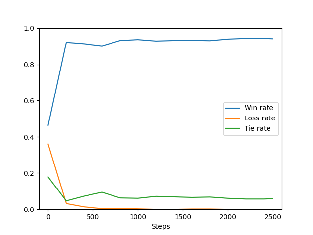
By about 1200 steps the model never loses to a random player and for the rest of training the fraction of ties decreases a bit.

If we ask the model to play against itself, it produces a tied game like this:

Perfect!

Footnotes