Voting is an odd thing. We all in some sense know that our individual votes are exceedingly unlikely to impact an election, but many of us find ourselves highly motivated to vote anyway. There are, of course, many reasons to vote — a sense of civic duty, an expression of political solidarity, or just as something to do brighten up a gloomy Tuesday morning. But let us set those aside for the time being. What if you were only concerned with having a non-negligible effect on the outcome of the election? Does it still make sense to vote?

First, what does it mean to have a non-negligible effect on the outcome? The strange thing about elections is that a single vote can only have any influence in one circumstance — when one candidate receives as many as the other plus one. In every other case any individual who voted for the victor could have abstained without affecting the outcome of the election. In those cases no individual decided the election. The outcome was decided by the aggregate behavior of the group rather than any individual action.

So if the only case in which an individual vote matters is when two candidates receive equal numbers of votes excluding your own, what is the probability of this happening? [¹]

Maximizing the likelihood of a decisive vote

Let’s start by putting an upper bound on the probability that a single vote could decide a presidential election. Since the president is elected by the electoral college, the voting patterns of the nation as a whole are not so relevant as votes within particular states. At the moment FiveThirtyEight predicts that Pennsylvania is the most likely to cast the decisive electoral college vote. So let’s focus on a Pennsylvanian voter in an election that is decided by Pennsylvania.

To further maximize the probability of this hypothetical scenario, let’s suppose that there are only two candidates on the ballot and the polls have Pennsylvania at exactly 50-50. Naturally there is some error in the polls so there is a distribution of outcomes that are consistent with a 50-50 polling result. Polling uncertainty can be broken into two components: statistical and systematic. Statistical uncertainty originates from the fact that polls measure only a subset of the population. So long as the sample size is moderately large, the central limit theorem guarantees that the statistical error has a Gaussian distribution; statistical error can be reduced simply by gathering a larger sample.

The systematic error is due to any biases in the polling methodology. Different subpopulations may have different response rates and different voting patterns. A naive random sample of the population can easily produce extremely biased results. [²] Much of the art of polling comes down to breaking the population into subpopulations, weighting their results appropriately, and correcting for any biases in response rates (along with estimating the turnout of each group, which we are completely ignoring here).

We shall assume that the total uncertainty in the polling result follows a Gaussian distribution. As we’ll discuss in more detail below, this is not generally correct for the systematic error, but so long as we’re considering outcomes that are not too far from the polling result, it is not a terrible approximation.

In this case we are interested in finding the probability that the outcome of the election is 50% to within one vote, in which case our lone vote will be decisive. Let’s denote the voting population by \(N\) and the polling uncertainty in raw votes by \(\sigma\). Then the probability that the outcome is within a single vote is

To make this a little easier to deal with, let’s normalize the variables by population. Rather than specifying the total uncertainty in raw numbers of votes, we shall instead consider the uncertainty as a fraction of the population, \(\widetilde{\sigma} \equiv \sigma / N\), and similarly the outcome of the vote as a fraction of the population, \(\widetilde{x} \equiv x / N\). The probability of an exactly equal outcome can then be written as

Since \(N\) is very large, we don’t in fact need to calculate this integral explicitly. The probability density function does not change very much over the narrow range \(\left[ 1/2(1 - 1/N), 1/2(1 + 1/N) \right]\), so we can approximate the probability by the value of the function at \(\widetilde{x} = 1/2\) times the width:

And since the width is simply \(\Delta \widetilde{x} = 1 / N\), we have

Pennsylvania has \(\sim\)9 million registered voters for the 2020 election (and we’ll assume that all registered voters vote). Let’s furthermore assume the polling uncertainty is 5%, which is the historical accuracy of polls in the general election. [³] With these numbers we have \(p \sim 9 \times 10^{-7}\), or slightly worse than one in a million.

The expected value of a decisive vote

These look like long odds! And indeed they are. But does this mean that we shouldn’t bother with voting? No! We can’t make that determination until we compare it with the value of casting the decisive vote relative to the cost of voting.

So how much is casting the decisive vote worth? It is hard to quantify this. We could ask, “How much would you be willing to pay to guarantee the outcome of a presidential election?” But that is probably not the right metric. After all, the median voter’s assets may be limited compared to the value of the outcome to them, and is certainly much less than its value to society as a whole. [⁴] As an alternative we could put its value at the total amount spent on campaigning. But this still likely a significant underestimate since campaign spending has diminishing returns. The marginal dollar spent on Biden or Trump’s campaign has a very weak impact on the likelihood of the outcome. We could imagine that if one could guarantee the outcome of an election by spending a certain amount, donors would be willing to fork up quite a bit more! Nevertheless, in a certain efficient markets sense, the amount of money spent on campaigning reflects a minimum bound on the value of a presidential candidate to at least some segments of society. [⁵]

So we shall have to satisfy ourselves with taking the value of the victory of a favored candidate to be the total campaign spending for the 2020 presidential election, which is about $11 billion. Given these assumptions, the expected value of casting a vote in a hypothetical toss-up Pennsylvania comes out to be \(\sim\)$9,800.

A realistic Pennsylvania

We’ve now found a best-case scenario for which the probability is casting the decisive vote is maximized. But as of this writing, Pennsylvania is not in a dead heat. FiveThirtyEight’s polling average has Biden up by 4.9% points in Pennsylvania. How does this affect the expected value?

Let’s call the polling differential \(\delta\). Then we have \(\widetilde{x} = 1/2 + \delta / 2\). With this change we now have the probability of casting the decisive vote as

Plugging in our assumed values we find that the probability of casting the decisive vote has now gone down to \(8 \times 10^{-7}\) with an expected value of $8300.

Accounting for the probability of voting in the tipping point state

So far we have simply assumed that Pennsylvania will cast the decisive vote. But there is no guarantee that this will happen. As of this writing, FiveThirtyEight gives Pennsylvania a 38% chance of being the tipping point state. [⁶]

So we should multiply the probabilities we found above by 30% to account for this. This means that a voter in Pennsylvania has a probability of \(3 \times 10^{-7}\) of deciding the presidential election, and we finally arrive at an expected value of \(\sim\)$3300.

As long as it costs you less than $3,300 to vote in this hypothetical scenario, you can at least go to the polls with the comfort that the expected value of your vote is quite high! (Even if the probability of the payoff is low.)

Voting in California

We can conclude that voting in Pennsylvania is worth it this election. But what if you live in California? Should you vote then?

FiveThirtyEight doesn’t explicitly provide the probability of California being the tipping point state, but only puts it at less than 1%. Let’s nevertheless assume the probability to be 1% in order to calculate an upper bound.

As of today FiveThirtyEight puts the polling differential in California at 29%. If we naively use the same method as above but now take the number of registered voters to be 21 million for California, the probability of casting a decisive vote in the presidential election is \(6 \times 10^{-11}\). Even assuming the prodigious payoff of $11 billion for pulling off that feat, the expected value of a California vote is a mere 62¢.

But how much can we trust these numbers? We can have more confidence in the numbers for Pennsylvania because a one-vote margin would require a polling error of a little less than a single standard deviation. But the probability of casting a decisive vote in California is so low because it would require an outlier of nearly six standard deviations. (That would be enough to even fool the notoriously conservative particle physics community, who consider an outlier of five standard deviations to be evidence of new physics.) If the uncertainties were in fact distributed as a Gaussian this would be a one in \(\sim\)500 million chance.

However, it is more likely that the errors only have an approximately Gaussian distribution near the mean. In the tails this approximation would prove much poorer. Here the uncertainty becomes dominated by the systematic uncertainty of the polls and there is no easy way to model this. One could make a good argument that the tails are fatter than a Gaussian, and hence that the odds of casting a decisive vote in California are much higher than we calculated above. (Perhaps the pollsters are missing an especially motivated demographic this cycle, and everyone else, assured in the certainty of California’s outcome, stays home that day.) But how much fatter should those tails be? Is the probability of California flipping a one a hundred million chance? A one in a million chance? A one in a thousand chance? The difficulty of systematic errors is that when they are large, you have no other choice but to deeply understand where they are coming from so that you can correct for them. Given that there have only been a few dozen presidential elections in the United States’s history, and each election is its own unique event anyway, it is very hard to estimate the probability of such exceedingly rare outcomes even to within an order of magnitude.

Is a third party vote wasted?

So if your vote is (probably) not going to be decisive in California, should you just vote for a third party candidate you better agree with instead? Naturally if your vote for a major party candidate is unlikely to be decisive, it is a fortiori the case that it will be less so for a candidate polling at just a few percent. But there are other thresholds falling short of victory which are nevertheless valuable. In particular a candidate who exceeds 5% of the national vote unlocks federal funding in the following election. Fortunately this grant has a specific monetary value so we don’t have to estimate an abstract “value to society” when calculating the expected value of this outcome — in 2020 this grant is about $100 million so we shall use that as the payoff.

We shall calculate the expected value of a vote for the highest polling third-party candidate in the 2020 presidential election, Libertarian nominee Jo Jorgensen. The RealClearPolitics polling average currently puts Jorgensen at 1.8%.

At this point we need to be a little careful with our choice of distribution. For polls that are close to 50% with \(\sim\)5% uncertainty, a Gaussian distribution is not terrible. But this is clearly a poor distribution for a candidate polling in single digits because it puts substantial odds that the candidate will achieve negative votes!

Unfortunately doing a principled derivation of the correct distribution would require a deep understanding of the the systematic uncertainties of these polls (which I certainly do not possess). So instead in the spirit of attempting to obtain an order of magnitude estimate, we shall instead fly by the seat of our pants. What we would like is a reasonable distribution of outcomes for Jorgensen that are consistent with a polling average of 1.8% and a \(\sim\)5% uncertainty on the major party candidates. Let us suppose that the 5% uncertainty on the outcomes of the major party candidates were purely statistical. If this were the case then it would correspond to some effective sample size \(N_{\textrm{eff}}\) that consisted of a truly representative sample of voters.

So what is the effective sample size? The sample itself is drawn from a binomial distribution, so its standard deviation is \(\sqrt{N_{\textrm{eff}}p(1-p)}\), and by the central limit theorem the uncertainty on an estimate of \(p\) is then \(\sqrt{p(1-p)/N_{\textrm{eff}}}\). Taking \(p \sim 1/2\) for the major party candidates (remember this is just an order of magnitude estimate!) we have

Solving for \(N_{\textrm{eff}}\) gives us an effective sample size of 100.

We can now turn to Bayesian analysis to derive the distribution of outcomes for Jorgensen. Essentially we want to find \(p(f_L | \mathcal{D})\), where \(f_L\) is the fraction of votes for Jorgensen and \(\mathcal{D}\) represents the data that went into the polls. From Bayes’s Theorem, this probability is equal to

What should the prior \(p(f_L)\) be? For simplicity we’ll use a beta distribution as it is the conjugate prior for a binomial distribution. But the beta distribution has two hyperparameters, \(\alpha\) and \(\beta\) — what should they be? Choosing a prior is oftentimes subjective. A common choice is to set \(\alpha = \beta = 1\) which makes this distribution uniform and therefore, in some sense, minimally informative. But this is not a good prior in this situation. It puts the probability of Jorgensen achieving 1% of the popular vote the same as her achieving 99%. This does not match my personal prior. I will pick \(\alpha = 1.1\) and \(\beta = 11.9\). The motivation for this choice is that there have been Libertarian candidates in the last twelve presidential elections and they have generally received around 1% of the popular vote. These values of \(\alpha\) and \(\beta\) correspond to a binomial distribution with twelve samples and a mean of 0.01. This produces a prior that looks like this:

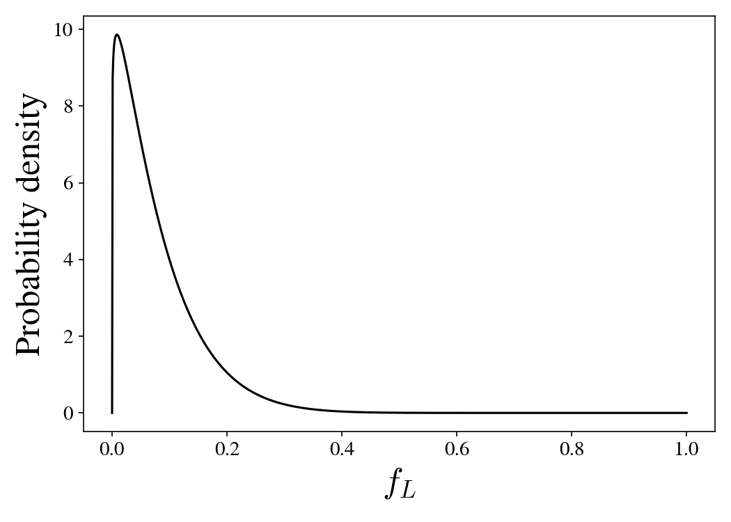
So, before seeing any polling data, we might reasonably expect that the Libertarian candidate will probably get a percentage point point or two, but we allow for a tail of possibilities where they end up doing exceptionally well and getting in the low double digits. One can quibble with the choice of prior, but any reasonable prior turns out not to have an enormous impact on the posterior distribution.

Now we can treat Jorgensen’s polling average as a sample from a binomial distribution with an effective sample size of 100 with \(\hat{f}_L N_{\textrm{eff}} = 1.8\) observed successes, where \(\hat{f}_L\) is the observed polling average of 1.8%. This then implies that the distribution of outcomes should look something like

where \(\textrm{B}\) is the beta function. (See this Wikipedia article for a derivation.) This produces a posterior distribution that looks like this:

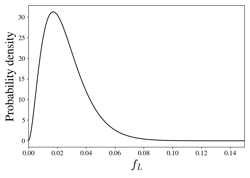
Based on this polling data we find that the posterior distribution is much more narrowly peaked around 1.8%.

Now that we have found a reasonable probability distribution describing Jorgensen’s outcomes, what is the probability of casting a decisive vote to bring her over the 5% threshold? We can write this probability as

where \(N\) is now the number of voters in the United States. Since \(N\) is very large we can make the following approximation:

Taking the number of voters in the United States to be \(\sim\)150 million we get a probability of \(p \sim 4 \times 10^{-8}\). Given the payoff of $100 million for exceeding the 5% threshold, the expected value of a third party vote is therefore \(\sim\)$4. So as you might expect, if you live in a swing state it makes more sense to vote for a major party candidate, but if you don’t, your expected payoff is larger if you vote third party. (Assuming, of course, that you identify more with that third party!)

The importance of polling uncertainty

Occasionally one sees estimates of the expected value of a vote that are many orders of magnitude below a penny. One calculation by Jason Brennan in The Ethics of Voting put the probability of casting a decisive vote in a close presidential election at somewhere around \(\sim \!\! 10^{-2660}\). Why are these calculations so far off from the calculation above? Brennan’s and similar calculations make a fundamental mistake by assuming that each voter is, in essence, flipping a coin with some known bias, and then calculating the probability of a 50-50 outcome from a binomial distribution. The issue with modeling votes this way is that it assumes that the mean of this distribution is known perfectly. Consequently, the width of this distribution is determined solely by the standard deviation of a binomial distribution. Brennan assumed a mean of 50.5%, and over the voting population of the United States this puts a 50-50 outcome as an outlier of more than a hundred standard deviations. Naturally the probability of observing such an event is ludicrously small.

But the correct model is not that we have flipped a hundred million coins with a bias of 50.5%. Rather, we have flipped a hundred million coins, but the bias of those coins could have been anywhere from 45.5% to 55.5%. And if the bias turned out to be very, very close to 50%, there is a reasonable chance of seeing a one-vote margin.

Ultimately we do not know what the true mean of the population is. So the width of this distribution is not determined by the statistical uncertainty of coin flips across an entire population, but by the uncertainty of the polls. Due to the difficulties around removing biases from polls, it is very hard to reduce polling uncertainties to below a few percent. And this few percent polling error makes all the difference when calculating the expected value of a vote. [⁷]

Postscript

This exercise is, of course, more an excuse to perform an order of magnitude calculation rather than exhortation to vote or not. Who goes to vote on the off chance that they will cast the deciding vote? Voting is principally an act of political expression and an exercise of civic duty, both binding the state closer to the citizen and the citizen closer to the state, with all the good and ill that entails. The decision to cast a vote is not, at its core, a rational calculation. I am reminded of Jane Jacobs on the subject of secession in Québec:

We care how our nation fares, care on a level deeper by far than concern with what is happening to the gross national product. Our feelings of who we are twine with feelings about our nation, so that when we feel proud of our nation we somehow feel personally proud. When we feel ashamed of our nation, or sorrow for it, the shame or the sorrow hits home.

These emotions are felt deeply by separatists, and they are felt equally deeply by those who ardently oppose separatists. The conflicts are not between different kinds of emotions. Rather, they are conflicts between different ways of identifying the nation, different choices as to what the nation is.

…

Trying to argue about these feelings is as fruitless as trying to argue that people in love ought not to be in love, or that if they must be, then they should be cold and hard-headed about choosing their attachment. It doesn’t work that way. We feel; our feelings are their own argument.

So, if your feelings so incline you, go vote! But if your feelings do not so incline you, you are now equipped to make your own coldly rational decision on the grounds of an expected value calculation!

A Jupyter notebook with the calculations in this post can be found here.

Footnotes