The paradox

Stein’s paradox is among the most surprising results in statistics. The basic idea is easily stated, but it is difficult to understand how it could possibly be true. The premise is this: suppose that I have a Gaussian distribution with a variance of unity and some mean which I don’t tell you. I then draw a single sample from this distribution, give it to you, and ask you to guess the mean. What do you do? Well, you don’t have a lot of information to go on here, so you just guess that the mean is the number I gave you. This is a good guess! (We will make the notion of a “good guess” a little more precise later on.)

No big surprise there. Now we play again, but this time, my distribution is a two-dimensional Gaussian. The covariance is the identity matrix (so this is equivalent to sampling from two independent one-dimensional Gaussians). But again I have not told you the mean (which is now a two-dimensional vector). Once more I draw a single sample from the distribution, hand it over to you, and ask you to guess the mean. You simply guess that the mean is the sample I have given you. Once more you have guessed well!

Now we do the same thing in three dimensions. I draw a single sample, hand it over to you, and ask you to guess the mean. Just as before, you guess that the mean is the sample I gave you. But this is no longer a good guess! Stein’s paradox is that if we play this game in three dimensions or more, a better guess is to say that the mean is this:

where \(D\) is the dimensionality of the Gaussian, and \(\mathbf{x}\) is the sample drawn from the distribution. This is the so-called “James-Stein estimator.”

Who would have thought! What is going on here?

What makes a guess good?

Before we go on, we should clarify exactly what we mean by a “good guess.” We are trying to do what is called “parameter estimation” in statistics — based on a sample from a distribution, we want to infer some underlying parameter (or parameters) of the distribution. (In this case the parameter we are interested in is the mean.) In order to quantify how good or bad our estimate is we choose a function called a “loss function.” There is some freedom in choosing a loss function, but the mean squared error is a common choice and has a lot of valuable properties. Stein’s paradox assumes that we are using the mean squared error. So if we guess that the mean is \(\hat{\mu}\) and the true value of the mean is \(\mu\), then the loss is

Now, of course, we need some rule to go from the sample \(\mathbf{x}\) to the estimate \(\hat{\mu}\). This rule is just a function of some kind, say, \(f(\mathbf{x})\). This function has the special name of an “estimator.” We can choose whatever function we want here. Our original guess was to just use \(f(\mathbf{x}) = \mathbf{x}\). But another choice here is to say \(f(\mathbf{x}) = \mathbf{x} + 7\), or \(f(\mathbf{x}) = \sin(\mathbf{x}) / \mathbf{x}^{71}\), or even just \(f(\mathbf{x}) = 31\). It doesn’t take much imagination to see that there are an infinite number of possible choices. But presumably some of these choices are better than others. How do we know which ones are good?

Statisticians use the concept of risk for this purpose. Risk is simply the expected value of your loss function. One thing that can be a little confusing is that the risk is a function of both your choice of estimator and the true value of the parameter itself. So in the original game where you’re guessing the mean of a one-dimensional Gaussian, the risk will be a function of whatever rule you decide to use and the actual, unknown value of the mean.

The fact that the risk is a function of the true value of the parameter makes things a little tricky. If you’re trying to decide between two estimators, you might find that one estimator works better for certain values that the parameter can take, and the other works better for others. As a dumb example, let’s go back to guessing the mean of a one-dimensional Gaussian. Our original estimator was \(\hat{\mu} = x\). But another, perfectly valid, estimator is \(\hat{\mu} = 7\). In other words we ignore the sample entirely and say that the mean is 7 no matter what. Generally this doesn’t seem like a smart thing to do. But if the mean turns out to actually be pretty close to 7, on average this will be the better guess! Specifically, the risk of our initial estimator is

And the risk on our second, dumb estimator is

As long as the true mean, \(\mu\), happens to be between 6 and 8, the dumb estimator of just saying 7 actually has lower risk!

Based on this example it might seem that we’re stuck. Since we don’t know the true value of the mean, we can’t generally say if one estimator is better than another. And indeed this is often the case. But there are certain situations where this is not true. If we have two estimators and one of them has a lower risk for any possible value the parameter can take, we can say that one is definitively better than the other. In statistical parlance, we say that the worse estimator is “inadmissable.”

In more precise terms, Stein’s paradox states that in three dimensions or more, the naive estimator (just guessing that the mean is \(\mathbf{x}\)) is inadmissable because the risk of the James-Stein estimator is lower for any possible mean I could choose.

What is the James-Stein estimator doing?

Before we can understand why the James-Stein estimator gives you a better guess than the naive estimator \(\textbf{x}\), we should understand what exactly it’s doing. The idea is that we take the naive guess \(\textbf{x}\) and then we scale it towards the origin by some amount. The factor by which we scale it is:

The ReLU function simply takes the maximum of its argument and zero, so this scale factor will be either positive or zero. Let’s suppose that it’s positive. In this case we scale it towards the origin more if the magnitude of the sample is smaller and less if it is lower. In the limit of \(|\textbf{x}| \to \infty\) we don’t change it at all and our guess reduces to the naive estimator \(\textbf{x}\).

In the other limit, if \(|\textbf{x}|\) is very small, then the ReLU function will kick in and just set the scale factor to zero. Hence anytime we get a sufficiently small sample we throw it out and just guess that the mean is zero instead. And all else being equal we will shrink our estimate more in higher dimensional spaces than in lower dimensional spaces.

So that is what the James-Stein estimator is doing. Why does it work? Before we can answer that we need to take a quick detour.

Samples in high dimensional spaces

High dimensional spaces are counterintuitive. One of the counteruintitive properties of high dimensional distributions is this: a sample from a symmetric high dimensional distirbution is highly likely to be further from the origin than the mean. Specifically, for an isotropic \(D\)-dimensional Gaussian, the difference between the average distance to a sample and the distance to the mean grows as \(\sim\)\(\sqrt{D}\).

It’s a little strange to put it this way, but isn’t so surprising with a little bit of thought. Even in two dimensions we can see that this is the case just by drawing it:

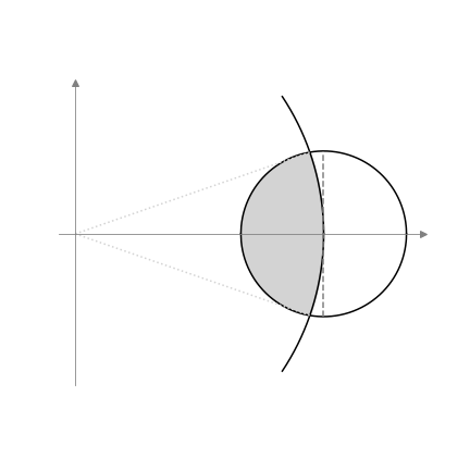
The shaded area of the circle is less than half the area, so we are less likely to choose a sample closer to the origin than the mean. What perhaps makes this counterintuitive is that in two dimensions a fairly large fraction of the circle is still shaded. But as the dimensionality increases, this fraction decreases exponentially. Once the dimensionality is even moderately large we are highly unlikely to sample a point in this shaded region.

One caveat here is that this effect decreases the larger the mean is. You can imagine that as we move the circle further away from the origin, the shaded fraction gets closer and closer to ½. So long as the mean is sufficiently large, the probability of sampling a point closer to the origin than the mean can be close to ½ even in high dimensional spaces; it just requires a very large mean. We can start to see here the connection to the James-Stein estimator, which also gets very close to the naive estimator \(\mathbf{x}\) as the mean (and hence \(|\mathbf{x}|\)) gets very large.

What we are doing by shrinking the estimate towards the origin is correcting for the tendency of the typical sample to be slightly further away from the origin than the mean. This correction allows us to reduce the overall risk of the estimate. [¹]

How arbitrary is the origin, really?

Stein’s paradox is particularly strange because there are actually two counterintuitive things going on:

1. The origin is arbitrary, so why does moving your estimate towards the origin help?
2. Why does this not work in one or two dimensions?

Let’s take a look at the first of these. A central principle in physics is that of relativity — coordinate systems are arbitrary, so the laws of physics must be valid in all of them. Surely this is also true in statistics as well. We can choose the origin to be wherever we like, so it cannot contain any information. But this sensible assertion is false. Statistics is not physics.

If we truly had no information about the mean, what value would the sample have? If it could really be anything then presumably its value would be exceedingly large. After all, there are a lot of numbers, almost all of them are too big to write down, and the mean could be absolutely any of them. But if we pick a sample and find that its distance from the origin is 3.72 there must be something fishy going on. Clearly we have, in fact, managed to embed some information in our choice of coordinate system. The only reason we have gotten out sensible values in our sample is because we have some prior as to where the mean is expected to be.

In fact, in the limit of no information \(| \mathbf{x} |\) will be infinitely large and the James-Stein estimator will reduce to the naive estimator, \(\mathbf{x}\). So it was our clever choice of origin that smuggled information into our estimator and allowed us to do better than the naive estimate.

It’s important to distinguish between the direction of the origin and the distance between the origin and the mean. The direction of the origin is unimportant. In fact, we could shrink our estimate in any direction and we would still get the benefits of the James-Stein estimator. The important thing is the distance between the origin and the mean — this is what has encoded some prior information that we can exploit to make a better prediction.

The bias-variance tradeoff

The way the James-Stein estimator works can be understood by looking at the bias-variance tradeoff. The bias-variance tradeoff states that the risk of an estimator can be decomposed into two components: a constant “bias” term, which reflects how far off the average value of the estimate is from the correct value; and an unbiased “variance” term, which accounts for the randomness of the sample.

The naive estimator \(\textbf{x}\) is unbiased but has a high variance. One reason that Stein’s paradox seems unnatural is that we tend to confuse unbiased estimators with estimators that minimize risk. But in high dimensional spaces, samples from an isotropic Gaussian encompass a tremendous volume. Although our naive estimate is unbiased it has very high variance.

What the James-Stein estimator does is scale the overall distribution towards the origin, thereby shrinking the volume of the distribution (and hence its variance), at the cost of introducing a little bit of bias. Although the estimator is now biased its overall risk is lower.

Deriving the James-Stein estimator geometrically

At this point we have some idea as to why shrinking the estimate towards the origin could be helpful, but we haven’t yet figured out why the specific form of the James-Stein estimator seems to work. To do this we’ll follow an argument presented by Brown & Zhao (2012).

Remember that the direction of the coordinate system is arbitrary. So let’s rotate into a new one where one axis points directly toward the mean, and the other \(D - 1\) axes are pointed in arbitrary (orthogonal) directions. (Of course, you can’t do this because you don’t know where the true mean is. But I do, and I’ve decided to help you out.) In this coordinate system the mean is just \((|\mu|, 0, \ldots, 0)\). Let’s write the sample in this coordinate system as \((\zeta_1, \zeta_2, \ldots, \zeta_D)\).

The loss for our guess can now be broken into two orthogonal components: one component, \((\zeta_1 - |\mu|)^2\), which tells us how far off our estimate is from the true value when it’s projected onto the correct direction of the mean; and a second component, \(\sum_{i=2}^D \zeta_i^2\), which tells us how far off our estimate is from this correct direction. Let’s call this second component the “residual” component and define it as

Our underlying distribution is isotropic, so rotating the coordinate system doesn’t change the fact that each coordinate \(\zeta_i\) is a sample from an independent one-dimensional Gaussian with unit variance. And if \(i > 1\) then the mean of this distribution is zero as well. \(\rho\) therefore follows a \(\chi\) distribution with \(D - 1\) degrees of freedom.

Let’s suppose that we’ve gone and chosen a sample from our distribution and by good fortune \(\zeta_1\) happens to be exactly equal to \(|\mu|\). In general the rest of the \(\zeta_i\) in the sample won’t be exactly zero and so \(\rho\) will be positive. If we plot \(\zeta_1\) on the \(x\)-axis and \(\rho\) on the \(y\)-axis, the situation will look like this:

The sample from our distribution is the point at the top right of the triangle. If we just use this sample as our estimate of the mean then the loss of this estimate will simply be the squared distance between the point and the bottom right corner of the triangle, or \(\rho^2\).

How can we transform the sample?

We only have two points in this problem: the origin, and the sample \(\textbf{x}\). By symmetry this means that the only way by which we can make an estimate is to choose a point somewhere on the line between the origin and \(\textbf{x}\). [²] In other words, you don’t actually know what direction any of the \(\zeta_i\) are in so you can’t simply move your guess down the right side of the triangle to reduce \(\rho\). The only direction you are allowed to move your sample is along the hypoteneuse of this triangle.

How should we transform the sample?

The beauty of the James-Stein estimator is that even though we are constrained to move the sample along the hypoteneuse, we can nevertheless reduce the distance between our guess and the true mean by shrinking it until the direction between our guess and the mean is perpendicular to the hypoteneuse.

Some simple geometry reveals that this new point is located at:

This is looking like the beginnings of the James-Stein estimator!

What exactly is \(\rho\)? Unfortunately \(\rho\) is random variable, but let’s represent it by some central point of its distribution. Now \(\rho\) follows a \(\chi\) distribution with \(D - 1\) degrees of freedom and the mode of this distribution is \(D - 2\). So if we simply represent this distribution by its mode, our estimator becomes

which is the James-Stein estimator without the ReLU.

To be clear, this is a very hand-wavey argument. Representing the entire distribution by a single point is not particularly sophisticated, and there is no special reason to choose to use the mode instead of the mean or median except that it happens to give an answer that corrseponds to the James-Stein estimator. [³]

Can we derive the James-Stein estimator rigorously?

Given how hand-wavey this argument was, you might wonder whether it’s possible to rigorously derive the James-Stein estimator by explicitly calculating the risk given the Gaussian and \(\chi\) distributions, and then finding the function that minimizes the risk using the calculus of variations. However this approach will not work. The reason is that the James-Stein optimizer does not actually minimize the risk! In fact, despite its fame, the James-Stein estimator is itself inadmissible.

As we’ll see below, we can improve our estimator by wrapping it in a ReLU function. But the ReLU function introduces some difficulties, because there is a very general theorem which states that any admissible estimator must be a Bayes estimator for some prior, or the limit of Bayes estimators. [⁴] This ends up implying that the estimator must be a smooth function and the ReLU function is not smooth. So while the James-Stein estimator beats the naive estimator \(\textbf{x}\), there exists some other estimator which beats it!

Recovering the ReLU

There is one last piece to tackle: the ReLU function. Where does that come from?

The ReLU has no effect on our estimate as long as \(|\textbf{x}| \geq D - 2\). This will generally be the case if \(|\mu|\) is large. But if \(|\mu|\) is small, then some of the points sampled will have \(|\textbf{x}| < D - 2\). If we were to just use the same scaling we derived above, we would reflect our estimate through the origin and make it negative! This estimate has a worse loss than an estimate at the origin.

The reason for this is that once we have shrunk the sample all the way down to the origin we have already traded away all the variance for bias. In other words, we started with an estimate that had no bias and high variance, and ended up with an estimate that had high bias and no varaiance. But if we were to keep going past the origin, we’d continue to increase the bias but would start to increase the variance as well! This is strictly worse than keeping our estimate at the origin, so we are better off clamping the estimate at zero with a ReLU function.

Why does Stein’s paradox not hold in two dimensions?

Let’s now turn to the second counterintuitive property of Stein’s paradox: what’s so special about three dimensions? It is not hard to see why the James-Stein estimator doesn’t help in one dimension — we arrived at the James-Stein estimator by separating the sample into two components, one along the direction to the true mean, and the other as a residual component perpendicular to the first. But in one dimension there is no residual component! By shrinking your estimate towards the origin you introduce some bias, but this is not counterbalanced by the reduction in variance.

But what about the two dimensional case? Here again we unfortunately must wave our hands. In the two dimensional case we do, in fact, reduce the variance by shrinking our estimate towards the origin, just not by enough to offset the bias we introduce. While the orthogonal component, \(\rho\), is not identically zero as it was in the one-dimensional case, it is strongly bunched up close to zero in the two dimensional case. The idea of the James-Stein estimator is to note that a certain proportion of a sample’s magnitude is due to a component orthogonal to the mean and to shrink the estimate to reduce that othogonal component somewhat. But if the magnitude of the orthogonal component is too small, this won’t always work. There are some values of the mean for which the James-Stein estimator is better, but others where it is worse. It is not the better estimator no matter what.

A digression on random walks

As an aside, there is a deep correspondence found by Lawrence Brown between random walks and the admissibility of the naive estimator, \(\textbf{x}\). Brown showed that the naive estimator is admissible if and only if a random walk returns to the origin an infinite number of times. Random walks in one or two dimensions do this, but random walks in three or more dimensions do not. At a high level this is because the random walk drifts away from the origin at a rate linear in the dimensionality of the space, but the volume subtended by the origin at a fixed distance decays exponentially with dimension. In one or two dimensions the volume subtended by the origin is large enough that you are guaranteed to eventually make your way back to it. But in higher dimensions, the volume subtended is smaller, so that as time progresses you are less and less likely to make your back and the probability approaches zero even in the limit of an infinite number of steps.

While rigorously proving this correspondance is non-trivial, both problems have at their core a comparison between the distance between a point and the origin and the volume of the unit sphere in the space.

There be dragons far from the origin

So that, at a high level, is why the James-Stein estimator works. We’ve been focused in this post on the simplest form of Stein’s paradox, which is a bit of a toy problem. But the artificiality of the problem shouldn’t befog us as to the significance of these ideas. The artificiality eases the analysis, but in fact the concepts that Stein’s paradox illustrates run much deeper through statistics and machine learning.

As we discussed earlier on, while we usually don’t think that there is anything special about our choice of origin, we do neveretheless use it to smuggle in some priors, even if those priors are weak and we perhaps do so unwittingly. This is also true of machine learning models, maybe even more so. For most machine learning models the origin really is special. For example, at the origin most garden-variety neural networks will exhibit particularly simple behavior — they will output all zeros indpendent of the input. [⁵] Any movement away from this special point will introduce complexity into the functional behavior of the model. Neural networks are, of course, non-linear, so it is not always true that points further from the origin in parameter space are more complicated, but it is generally true.

Most ML practitioners appreciate that techniques like L2 regularization have the effect of making models simpler, and therefore less likely to overfit. But Stein’s paradox dramatically illustrates the relationship between the risk of an estimate and the dimensionality of the space — in high dimensional spaces there is much more volume further away from the origin than closer to it. We are oftentimes better off introducing bias in order to reduce variance because in high dimensional spaces shrinking a small amount towards the origin reduces an enormous volume of parameter space. In other words, for a large machine learning model, there are vastly more ways to overfit than there are to underfit so we should bias our models towards underfitting because that is a simpler problem to solve than overfitting. (Or maybe to put it another way, underfitting is a small number of problems, whereas overfitting is a stupendous number of problems.)

This phenomenon can manifest itself during neural network training. Suppose we have converged on a local minimum in the loss landscape after training with some varaint of stochastic gradient descent. At convergence there will be equality between the stochastic component of SGD, for which the random walk is causing the parameters to drift away from the minimum, and the true gradient, which is pushing the parameters towards the minimum. [⁶] At this point the neural network is wandering on some high-dimensional ellipsoid around the minumum. But by the nature of high dimensional spaces, the neural network will always be further from the origin than the minimum, and therefore on the side of too much complexity. Thus this converged model will always slightly overfit.

The further the model recedes from the origin, the more inexplicable its functional behavior can become. The moral of this story is that far from the origin there be dragons, and in a high dimensional space, moving just a little further away from the origin introduces lots and lots of dragons. The James-Stein estimator advises you to stay close to the origin to keep your risk down and the dragons at bay.

Footnotes